Plotting the dynamics in 1D¶

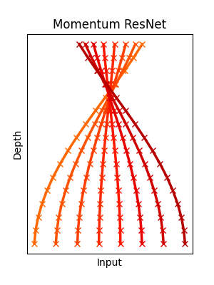
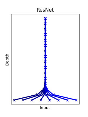
This example compares the dynamics of a ResNet and a Momentum ResNet. We try to learn a mapping with crossing trajectories. Trajectories corresponding to the ResNet fail to cross. On the opposite, the Momentum ResNet learns the desired mapping.

Michael E. Sander, Pierre Ablin, Mathieu Blondel, Gabriel Peyre. Momentum Residual Neural Networks. Proceedings of the 38th International Conference on Machine Learning, PMLR 139:9276-9287

# Authors: Michael Sander, Pierre Ablin
# License: MIT
import copy

import torch
import torch.nn as nn
import numpy as np
import matplotlib.pyplot as plt
import torch.optim as optim

from momentumnet import MomentumNet
from momentumnet.toy_datasets import make_data_1D

Fix random seed for reproducible figures¶

torch.manual_seed(1)

Out:

<torch._C.Generator object at 0x7f4846338a90>

Parameters of the simulation¶

hidden = 16
n_iters = 15
gamma = 0.99
d = 1

Defining the functions for the forward pass¶

function = nn.Sequential(nn.Linear(d, hidden), nn.Tanh(), nn.Linear(hidden, d))
function_res = copy.deepcopy(function)

Defining our models¶

mom_net = MomentumNet(
    [
        function,
    ]
    * n_iters,
    gamma=gamma,
    init_speed=0,
)
res_net = MomentumNet(
    [
        function_res,
    ]
    * n_iters,
    gamma=0.0,
    init_speed=0,
)

Training our models to learn a non-homeomorphic mapping¶

def h(x):
    return -(x ** 3)


def Loss(pred, x):
    return ((pred - h(x)) ** 2).mean()


optimizer = optim.SGD(mom_net.parameters(), lr=0.01)


for i in range(301):
    optimizer.zero_grad()
    x = make_data_1D(200)
    pred = mom_net(x)
    loss = Loss(pred, x)
    loss.backward()
    optimizer.step()

optimizer = optim.SGD(res_net.parameters(), lr=0.01)


for i in range(2001):
    optimizer.zero_grad()
    x = make_data_1D(200)
    pred = res_net(x)
    loss = Loss(pred, x)
    loss.backward()
    optimizer.step()

Plotting the output¶

n_plot = 8

num_plots = n_plot

plt.figure(figsize=(3, 4))
colormap = plt.cm.gist_ncar
plt.gca().set_prop_cycle(
    plt.cycler("color", plt.cm.jet(np.linspace(0.8, 0.95, num_plots)))
)

x_ = make_data_1D(n_plot)
x = np.linspace(-1, 1, n_plot)
x_ = torch.tensor(x).view(-1, d).float()
x_axis = np.arange(0, n_iters + 1)

preds = np.zeros((n_iters + 1, n_plot))

preds[0] = x_[:, 0]

for i in range(1, n_iters + 1):
    mom_net = MomentumNet(
        [
            function,
        ]
        * i,
        gamma=gamma,
        init_speed=0,
    )
    with torch.no_grad():

        pred_ = mom_net(x_)
        preds[i] = pred_[:, 0]

plt.plot(preds, x_axis, "-x", lw=2.5)
plt.xticks([], [])
plt.yticks([], [])
plt.title("Momentum ResNet")
plt.ylabel("Depth")
plt.xlabel("Input")
plt.show()

num_plots = n_plot

plt.figure(figsize=(3, 4))
colormap = plt.cm.gist_ncar
plt.gca().set_prop_cycle(
    plt.cycler("color", plt.cm.jet(np.linspace(0.0, 0.1, num_plots)))
)

x_axis = np.arange(0, n_iters + 1)

preds_res = np.zeros((n_iters + 1, n_plot))

preds_res[0] = x_[:, 0]
for i in range(1, n_iters + 1):
    res_net = MomentumNet(
        [
            function_res,
        ]
        * i,
        gamma=0.0,
        init_speed=0,
    )

    with torch.no_grad():
        pred_ = res_net(x_)
        preds_res[i] = pred_[:, 0]

plt.plot(preds_res, x_axis, "-x", lw=2.5)
plt.xticks([], [])
plt.yticks([], [])
plt.title("ResNet")
plt.ylabel("Depth")
plt.xlabel("Input")
plt.show()

Total running time of the script: ( 0 minutes 27.402 seconds)

Gallery generated by Sphinx-Gallery